unique index vs non-unique index

Question:

What is between between “unique index vs non-unique index”. Which one is faster. The customer using non-unique and sql is getting delay If we change tp non-unique. Is it work ?

Answer:

Indexes can be unique or non-unique. Unique indexes guarantee that no two rows of a table have duplicate values in the key column (or columns). Non-unique indexes do not impose this restriction on the column values.

Oracle recommends that unique indexes be created explicitly, using CREATE UNIQUE INDEX. Creating unique indexes through a primary key or unique constraint is not guaranteed to create a new index, and the index they create is not guaranteed to be a unique index.

It is just that in a unique index, the rowid is not considered “part of the key” and in a non-unique index “the rowid is considered part of the key”.

From Performance point of view:

The optimizer can look at an index that is unique and check, if you use “where x =:x and y = :y and ….” I’m going to get ONE row back, I can cost that much better”

If the index is non-unique, the optimizer will perform , index range scan, he is going to get 0..N rows back” and it’ll cost it differently.

So, a unique index will affect the generated plan — it is more information for the optimizer to grab onto.

If the data must be UNIQUE, you should use a UNIQUE constraint – not an index. We will take care of the index for you. If the constraint is not deferrable, we’ll create a unique index for you. If the constraint is deferrable — we’ll use a non-unique index.
Non-Unique indexes have various “overheads” when compared to Unique Indexes

Will examine two key differences today:

  • Extra byte required per index row entry
  • Index requires additional consistent reads and latch gets

Reading a Non-Unique Index is more expensive in terms of consistent reads and latches.

List Oracle SQL Hints

Below lists Oracle SQL hints:

RBO基于规则的优化器access paths优先级

RBO基于规则的优化器access paths优先级:

RBO Path 1: Single Row by Rowid

RBO Path 2: Single Row by Cluster Join

RBO Path 3: Single Row by Hash Cluster Key with Unique or Primary Key

RBO Path 4: Single Row by Unique or Primary Key

RBO Path 5: Clustered Join

RBO Path 6: Hash Cluster Key

RBO Path 7: Indexed Cluster Key

RBO Path 8: Composite Index

RBO Path 9: Single-Column Indexes

RBO Path 10: Bounded Range Search on Indexed Columns

RBO Path 11: Unbounded Range Search on Indexed Columns

RBO Path 12: Sort Merge Join

RBO Path 13: MAX or MIN of Indexed Column

RBO Path 14: ORDER BY on Indexed Column

RBO Path 15: Full Table Scan


注意在不违反如上优先级的前提下,若有2个优化级一样的索引可用,则RBO会选择晚建的那个索引, 解决方法是重建你想要让RBO使用的那个索引,或者使用CBO…….. 😆


在Oracle 10g以后虽然RBO (optimizer_mode=RULE)仍可用,但是不受官方的支持认可。

Histograms: An Overview

NOTE: This article was originally created for version 7.3. Conceptually the ideas presented are
the same as in later versions but implementation details may have changed or have
been enhanced.

Histograms
==========

For uniformly distributed data, the cost-based approach makes fairly accurate
guesses at the cost of executing a particular statement. However, when the
data is not uniformly distributed, the optimizer cannot accurately estimate
the selectivity of a query. Beginning in release 7.3, for columns which do not
have uniform data distribution, Oracle will allow you to store histograms
describing the data distribution of a particular column.

When to Use Histograms
———————-

Histograms are stored in the dictionary and computed by using the DBMS_STATS
command on a particular column. Therefore, there is a maintenance and space
cost for using histograms. You should only compute histograms for columns
which you know have highly-skewed data distribution.

When to Not Use Histograms
————————–

Also, be aware that histograms, as well as all optimizer statistics, are
static. If the data distribution of a column changes frequently, it is
necessary to recompute the histogram for a given column. Histograms are not
useful for columns with the following characteristics:

  o all predicates on the column use bind variables
  o the column data is uniformly distributed
  o the column is not used in WHERE clauses of queries
  o the column is unique and is used only with equality predicates

How to Use Histograms
———————

Create histograms on columns that are frequently used in WHERE clauses of
queries and have a highly-skewed data distribution. You create a histogram
by using the ANALYZE and DBMS_STATS TABLE command for later versions. For example, if you want to create a 10-bucket histogram on the SAL column of the EMP table, issue the following
statement:

    DBMS_STATS.GATHER_TABLE_STATS (NULL,’EMP’, method_opt => ‘FOR COLUMNS sal SIZE 10’);
    ANALYZE TABLE emp COMPUTE STATISTICS FOR COLUMNS sal SIZE 10;

The SIZE keyword states the maximum number of buckets for the histogram.
You would create a histogram on the SAL column if there were an unusual
number of employees with the same salary and few employees with other
salaries.

The ‘FOR’ clause can be used with either COMPUTE STATISTICS or ESTIMATE
STATISTICS.  The following clauses can be used with the ANALYZE TABLE command:

    FOR TABLE  
        collect table statistics for the table
    FOR ALL COLUMNS
        collect column statistics for all columns in the table
    FOR ALL INDEXED COLUMNMS   
        collect column statistics for all indexed columns in the table
    FOR COLUMNS
        collect column statistics for the specified columns
    FOR ALL INDEXES
        all indexes associated with the table will be analyzed
    SIZE
        specifies the maximum number of partitions (buckets) in the
        histogram.
         Default value:    75
         Range of values:  1 – 254

 For DBMS_STATS, syntax is the following:

method_opt

Accepts:

      FOR ALL [INDEXED | HIDDEN] COLUMNS [size_clause]
    *

      FOR COLUMNS [size clause] column|attribute [size_clause] [,column|attribute [size_clause]…]

size_clause is defined as size_clause := SIZE {integer | REPEAT | AUTO | SKEWONLY}

– integer : Number of histogram buckets. Must be in the range [1,254].
– REPEAT : Collects histograms only on the columns that already have histograms.
– AUTO : Oracle determines the columns to collect histograms based on data distribution and the workload of the columns.
– SKEWONLY : Oracle determines the columns to collect histograms based on the data distribution of the columns.

For 11.2, there is following additional parameter:

– extension : can be either a column group in the format of (column_name, Colume_name [, …]) or an expression

In 10g and 11g, the default is FOR ALL COLUMNS SIZE AUTO. The default value can be changed using the SET_DATABASE_PREFS Procedure, SET_GLOBAL_PREFS Procedure, SET_SCHEMA_PREFS Procedure and SET_TABLE_PREFS Procedure.

Choosing the Number of Buckets for a Histogram
———————————————-

The default number of buckets is 75. 10g onwards, the default value is FOR ALL COLUMNS SIZE AUTO.  This value provides an appropriate level of detail for most data distributions. However, since the number of buckets in the histogram, the sampling rate, and the data distribution all affect
the usefulness of a histogram, you may need to experiment with different
numbers of buckets to obtain the best results.

If the number of frequently occurring distinct values in a column is relatively
small, then it is useful to set the number of buckets to be greater than the
number of frequently occurring distinct values.

Viewing Histograms
——————

You can find information about existing histograms in the database through the
following data dictionary views:

    USER_TAB_HISTOGRAMS, ALL_TAB_HISTOGRAMS, and DBA_TAB_HISTOGRAMS.
    USER_PART_HISTOGRAMS, ALL_PART_HISTOGRAMS, and DBA_PART_HISTOGRAMS.
    USER_SUBPART_HISTOGRAMS, ALL_SUBPART_HISTOGRAMS, and DBA_SUBPART_HISTOGRAMS.

The number of buckets in each column’s histogram is found in these dictionary views :

 o USER_TAB_COL_STATISTICS, ALL_TAB_COL_STATISTICS,DBA_TAB_COL_STATISTICS
   (extracted from USER_TAB_COLUMNS, ALL_TAB_COLUMNS, and DBA_TAB_COLUMNS)
 o USER_PART_COL_STATISTICS,ALL_PART_COL_STATISTICS, DBA_PART_COL_STATISTICS,
 o USER_SUBPART_COL_STATISTICS, ALL_SUBPART_COL_STATISTICS, DBA_SUBPART_COL_STATISTICS

These views have the same definition.

DBA_TAB_HISTOGRAMS

This view lists histograms on columns of all tables.

Column name           Represents This
———————————————————
OWNER                 Owner of table
TABLE_NAME            Table name
COLUMN_NAME           Column name
ENDPOINT_NUMBER       Endpoint number
ENDPOINT_VALUE        Normalized endpoint values for this bucket

DBA_TAB_COLUMNS

This view contains information which describes columns of all tables.
(NOTE: Views and clusters, although included in this view are not relevant
 to histograms.)

Column Name           Represents This
———————————————————-
OWNER                 Owner of table
TABLE_NAME            Table name
COLUMN_NAME           Column name
DATA_TYPE             Datatype of the column
DATA_LENGTH           Length of the column
DATA_PRECISION        Precision for NUMBER or FLOAT datatypes
DATA_SCALE            Digits to right of decimal
NULLABLE              NULL allowable?
COLUMN_ID             Sequence no. of column
DEFAULT_LENGTH        Length of default value
DATA_DEFAULT          Default value
NUM_DISTINCT          Number of distinct values for the column
LOW_VALUE             Smallest value for the column, expressed in hex
                        for the internal representation ofthe first 32
                        bytes of the value
HIGH_VALUE            Highest value for the column, expressed in hex for
                        the internal representation of the first 32 bytes
                        of the value
DENSITY               Density of the column (a measure of how distinct
                        the values are)
NUM_NULLS             The number of columns with null value
NUM_BUCKETS           The number of buckets in the histogram
LAST_ANALYZED         The date that analyze was last run on the table
SAMPLE_SIZE           The amount of data sampled

The column LAST_ANALYZED is useful in determining the last time
statistics, with or without histograms, were computed.  This is
often important to assess the reason for cost-based optimizer’s
choices of execution paths.  All tables involved in a query must be
regularly analyzed as data changes.

Gather DBMS_STATS Default parameter

What are the default parameter values ?

   select dbms_stats.get_param('cascade') from dual;
   select dbms_stats.get_param('degree') from dual;
   select dbms_stats.get_param('estimate_percent') from dual;
   select dbms_stats.get_param('method_opt') from dual;
   select dbms_stats.get_param('no_invalidate') from dual;
   select dbms_stats.get_param('granularity') from dual;


DEFAULT PARAMETER

DBMS_STATS.AUTO_CASCADE
NULL
DBMS_STATS.AUTO_SAMPLE_SIZE
FOR ALL COLUMNS SIZE AUTO
DBMS_STATS.AUTO_INVALIDATE
AUTO

Skip Scanning of Indexes Advantages

What is skip scanning?


In prior releases, a composite index would be used to retrieve the records, if the index prefix (leading) column was included in the predicate of the statement. With Oracle9i, the optimizer can use a composite index even if the prefix column value is not known. The optimizer uses an algorithm called skip scanning to retrieve ROWIDs for values that do not use the prefix column.


How does a skip scan work?


During a skip scan, the B*-tree is probed for each distinct value in the prefix column. Under each prefix column value, the normal search algorithm takes over. The result is a series of searches through subsets of the index, each of which appears to result from a query using a specific value of the prefix column. However, with the skip scan, the value of the prefix column in each subset is obtained from the initial index probe rather than from the command predicate.

The optimizer uses the statistics to determine whether a skip scan retrieval would be more efficient than a full table scan, or other possible retrieval paths, when parsing SQL statements.


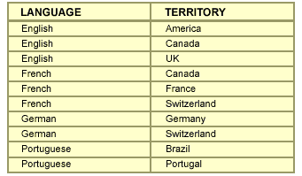
Suppose a composite index exists on the two columns, LANGUAGE andTERRITORY, with LANGUAGE as the prefix column. The data values stored in the underlying table result in the combinations of values in the table, as shown below. Each combination can occur multiple times in the table and the resulting index.
In previous releases without the skip scan algorithm, a query on a value in theTERRITORY column was forced to execute a full table scan or a fast full index scan. If the query were more common, then you might have needed to add a new index on the TERRITORY column alone. This new index, could negatively impact the performance of DML on the table.
The skip scan solution provides an improvement without the need for the second index. While not as fast as a direct index look up, the skip scan algorithm is faster than a full table scan in cases where the number of distinct values in the prefix column is relatively low.


Note: The skip scan feature cannot be turned on and off by the user. This feature is always on and is transparent to the users.


What are the advantages of skip scanning?

  • Skip scans reduce the need to add an index to support occasional queries that do not reference the prefix column of an existing index. This can be useful when high levels of DML activity is expected to degrade because of the existence of too many indexes used to support infrequent queries.
  • The algorithm is also valuable in the cases where there are no clear advantages as to which column to use as the prefix column in a composite index.
  • The prefix column should be the most discriminating, but also the most frequently referenced in queries. Sometimes, these two requirements are met by two different columns in a composite index, forcing a compromise or the use of multiple indexes. Skip scanning helps to overcome these problems.

沪ICP备14014813号-2

沪公网安备 31010802001379号